Small Edge, Small Bet
A manager can be right about the business and wrong about how much money to put into it. Kelly is a way of taking that problem seriously. Think of it as humility with a position size attached.
Imagine a manager with ten stocks, each worth 10% of the portfolio. The research is deep. The businesses are exciting. The first three years are excellent. The manager gets interviews. Investors get interested. The position sizes start to look like proof of skill.
Then several holdings fall together. The manager explains that the market has confused volatility with risk. Investors discover that the distinction is less comforting when half their money is gone.
My view is that a dominant failure in investment management is overbetting a small edge as if it were a large one. You can find good ideas, do honest work, and still build a portfolio that asks those ideas to carry far too much weight.
The useful question is how much your advantage supports risking, after allowing for the possibility that you have overstated it.
The man behind the formula
John Larry Kelly Jr. was a physicist from Texas who worked at Bell Labs. His name became famous in investing because of a 1956 paper about information and betting. It grew out of the world of communications research, where a signal can be useful without being perfect.
Kelly considered a bettor receiving useful information about sporting outcomes over a private wire. Better information gave the bettor an advantage. It did not make every tip correct. Betting everything on each tip would eventually turn one wrong message into a complete loss.
His question was how to use an advantage to grow wealth over repeated bets. The answer connected the size of the bet to the quality of the information and the payoff. A small advantage supported a small bet. More information did not grant permission to ignore the possibility of being wrong.
That is an awkward message for an industry that often sells certainty by the hour.
Winning more often can still make you poorer
Start with a deliberately simple game. You win your stake or lose your stake. Each bet is independent. Your true chance of winning is 52%. There are no costs, and money left aside earns no interest.
The full Kelly stake is 4% of your current bankroll. Quarter Kelly is 1%. Now suppose someone decides that 10% sounds more appropriate for a high-conviction idea.
Give all three strategies exactly the same 1,000 outcomes: 520 wins and 480 losses. Start each with $100.
| Stake on each bet | Ending wealth |
|---|---|
| 1%: quarter Kelly | $142 |
| 4%: full Kelly | $223 |
| 10%: overbet | $36 |
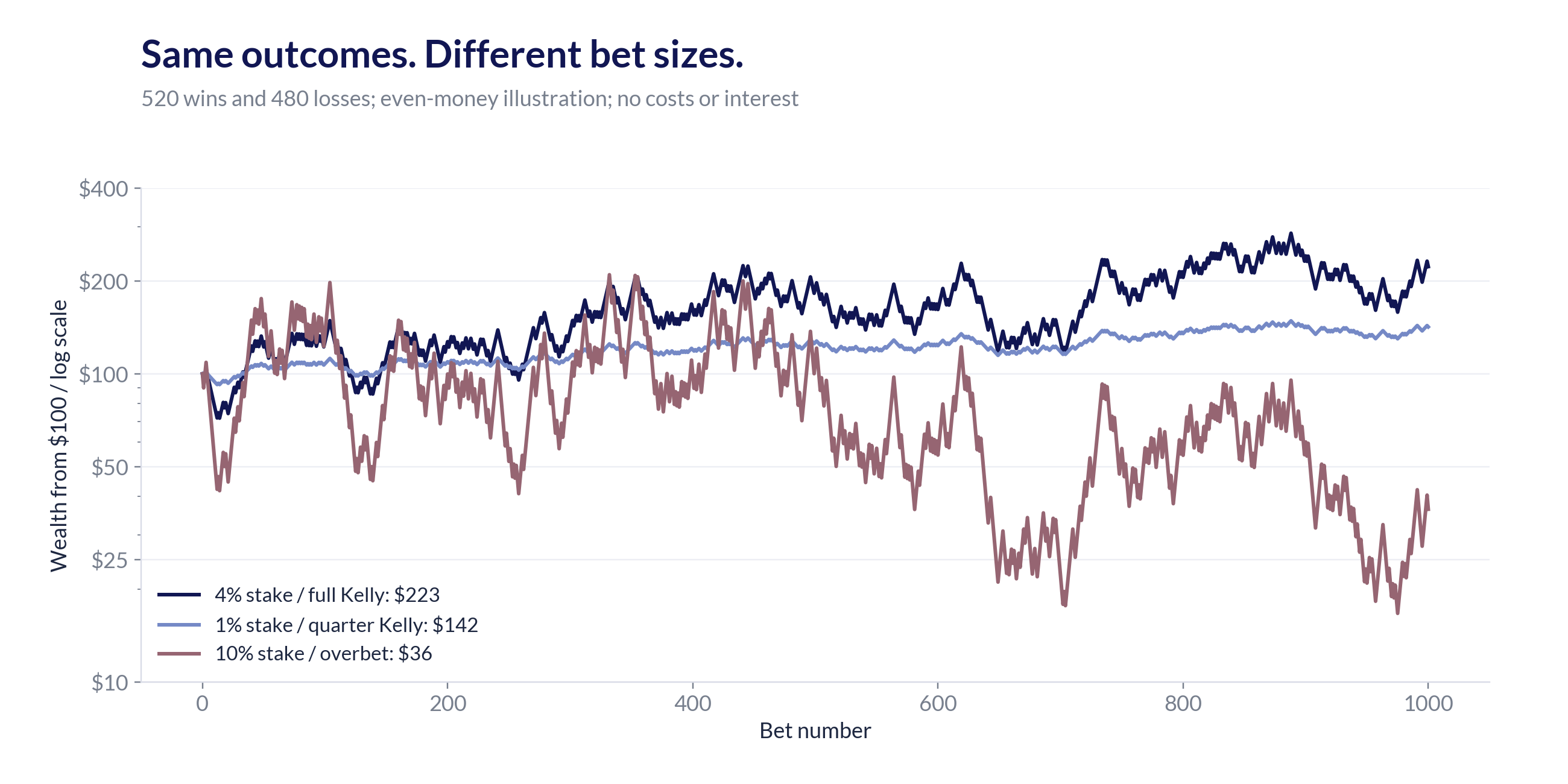
The oversized bettor wins more often than he loses and destroys almost two-thirds of his wealth. He has an edge. He simply demands too much from it.
Losses change the base on which future gains compound. Gain 10% and then lose 10%, and $100 becomes $99. Repeat that problem often enough and the damage grows. In this game, a 10% stake has negative expected log growth despite its positive expected profit per dollar bet. Repeated overbetting can drive wealth toward zero.
The research can be right. The bet can still be wrong.
Why use quarter Kelly?
Full Kelly maximizes expected long-run log growth under the model's assumptions. It does not promise a comfortable ride. It also assumes you know the advantage you are feeding into the formula.
That assumption deserves more attention than the formula.
Suppose you estimate a 55% chance of winning an even-money bet. Full Kelly says 10%. But the true chance is 52%, so the true full Kelly stake is only 4%. You are betting two and a half times that amount because your estimate was three percentage points too high.
Three points is a modest forecasting error. The sizing error is enormous.
Quarter Kelly means taking one-quarter of the full stake implied by your estimate. In this example, that is 2.5%: a quarter of the estimated 10%, rather than a quarter of the true 4% that you do not know. The smaller stake creates room for estimation error.
It also has a cost. If your estimate is exactly right, smaller bets give up some expected growth. In the simple game above, true quarter Kelly ends with less money than true full Kelly. The benefit is a less punishing exposure to being wrong, not a free increase in return.
Quarter Kelly is useful because public-equity forecasts come with uncertain payoffs, uncertain odds, and uncertain relationships between holdings. A forecast can look precise because someone put it in a spreadsheet. The spreadsheet did not collect more evidence.
Nor is one-quarter a magic safety setting. If the supposed edge is negative, a smaller bad bet is still a bad bet. Sometimes the sensible position is zero.
What would a 10% position require?
Managers with ten or twenty stocks often treat a 10% position as an ordinary expression of conviction. It is worth asking what assumptions could support that weight.
In the same independent, even-money game, the required true win probabilities would be:
| Bankroll stake | Full Kelly | Half Kelly | Quarter Kelly |
|---|---|---|---|
| 5% | 52.5% | 55% | 60% |
| 10% | 55% | 60% | 70% |
If a 10% stake is supposed to be quarter Kelly in that game, you need a genuine 70% chance of winning. Feeling 70% confident is not the same thing. You would need evidence that forecasts like yours actually come true at roughly that rate under comparable conditions.
Even a record of 55 correct calls out of 100 independent trials leaves a wide range of plausible underlying accuracy. A winning record is a start, not a license to enter your favorite probability and press “calculate.”
These are bankroll stakes in a toy game, not a conversion table for stock weights. A stock can rise 40%, fall 40%, double, or become worthless. Its payoff matters. So do the other positions.
Change the game to a stock that can only gain or lose 40%, with the rest in zero-interest cash. A 10% stock weight would be quarter Kelly at a 58% win probability. Change those payoffs or add correlated holdings, and the answer changes again.
A 10% stock position does not reveal a unique win probability. It does reveal a need to explain the expected gain, the possible loss, the evidence behind both, and the risk already sitting elsewhere in the portfolio.
“We know the company well” leaves most of that question unanswered.
Ten stocks can be the same bet ten times
A portfolio can own different businesses and depend on the same economic outcome.
An online retailer, a software company, a digital lender, and an advertising platform have different products. Their shares may still depend on cheap funding, strong consumer demand, generous valuations, and investors' willingness to pay today for profits far in the future.
The company descriptions differ. The bad day can be the same.
In a simple equal-weight model, ten stocks with equal risk and 60% pairwise correlation have the same variance reduction as about 1.56 independent bets. Twenty stocks at the same correlation get you to about 1.61. Doubling the names barely improves the diversification.
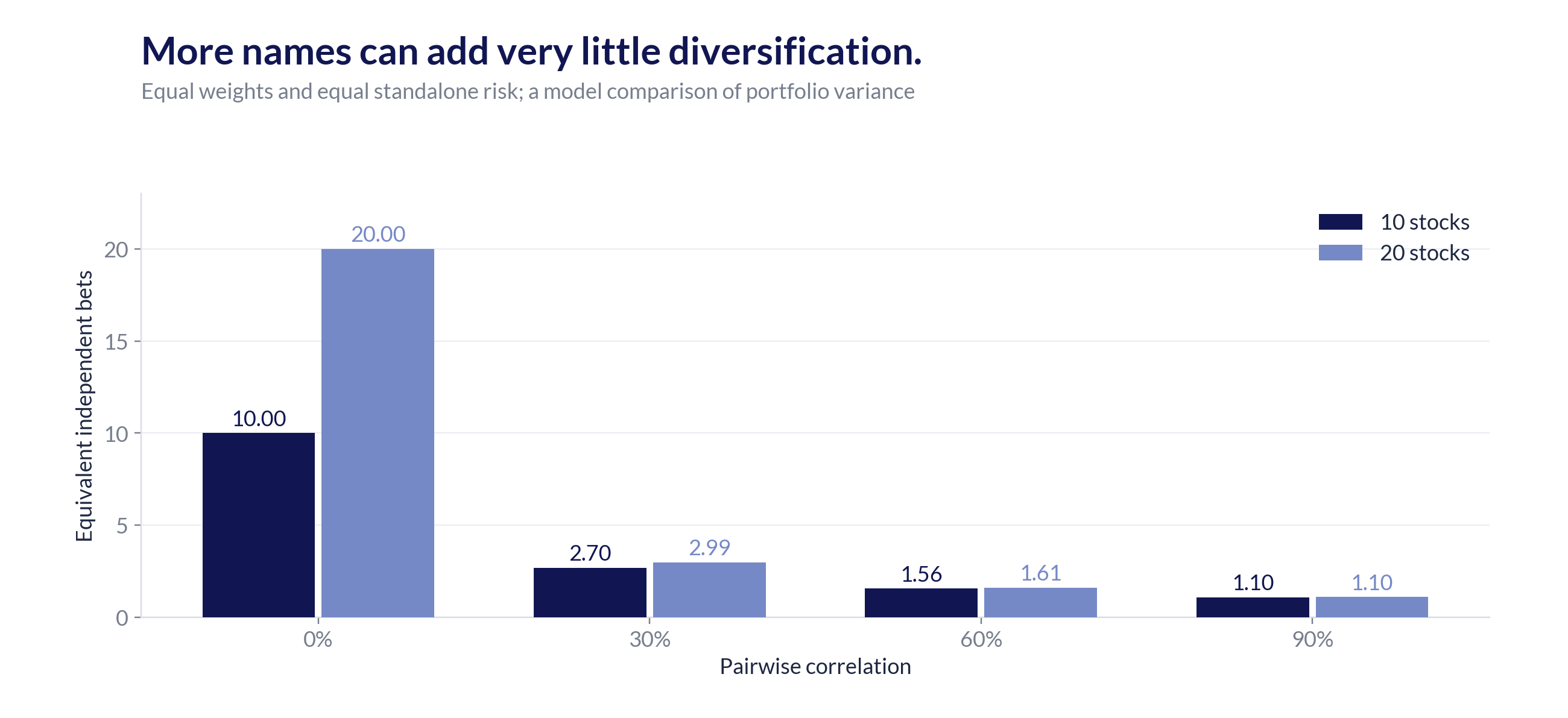
That matters for Kelly. You cannot size each stock as though the rest of the portfolio does not exist. A position may look small on its own while adding to a very large shared bet.
Adding another growth stock does not necessarily diversify a growth portfolio. Sometimes it just gives the existing risk a new logo.
Three good years, then a much harder conversation
Here is a hypothetical ten-stock fund against actual annual S&P 500 returns including dividends for 2011–2025, using the NYU historical compilation.
Each stock has a modest positive edge in the model: a 53% chance of outperforming the benchmark. Wins and losses are large, and the stocks share risk. Their modeled residual outcomes have 60% pairwise correlation. The manager puts 10% in each stock.
The first three fund returns are 18.4%, 34.4%, and 42.7%. The initial $100 becomes $227. That is a perfectly serviceable foundation for a compelling marketing deck.
By the end of 2015 it has fallen to $149. A later run takes it to $562 in 2021. The 2022 decline cuts it to $276. By 2025 it has recovered to $645, versus $708 for the benchmark.
This is an authored good-then-bad path, not a randomly selected historical manager or a forecast. The model does not make every concentrated portfolio fail. It shows how a real positive edge can coexist with a badly oversized portfolio.
The lighter line uses the same picks at model quarter Kelly, with the rest in the S&P benchmark. Under these particular assumptions, the optimal full sleeve is about 23.3% of capital, and its quarter-sized sleeve is about 5.8%. The manager's 100% sleeve is roughly 4.3 times the model's full Kelly size.
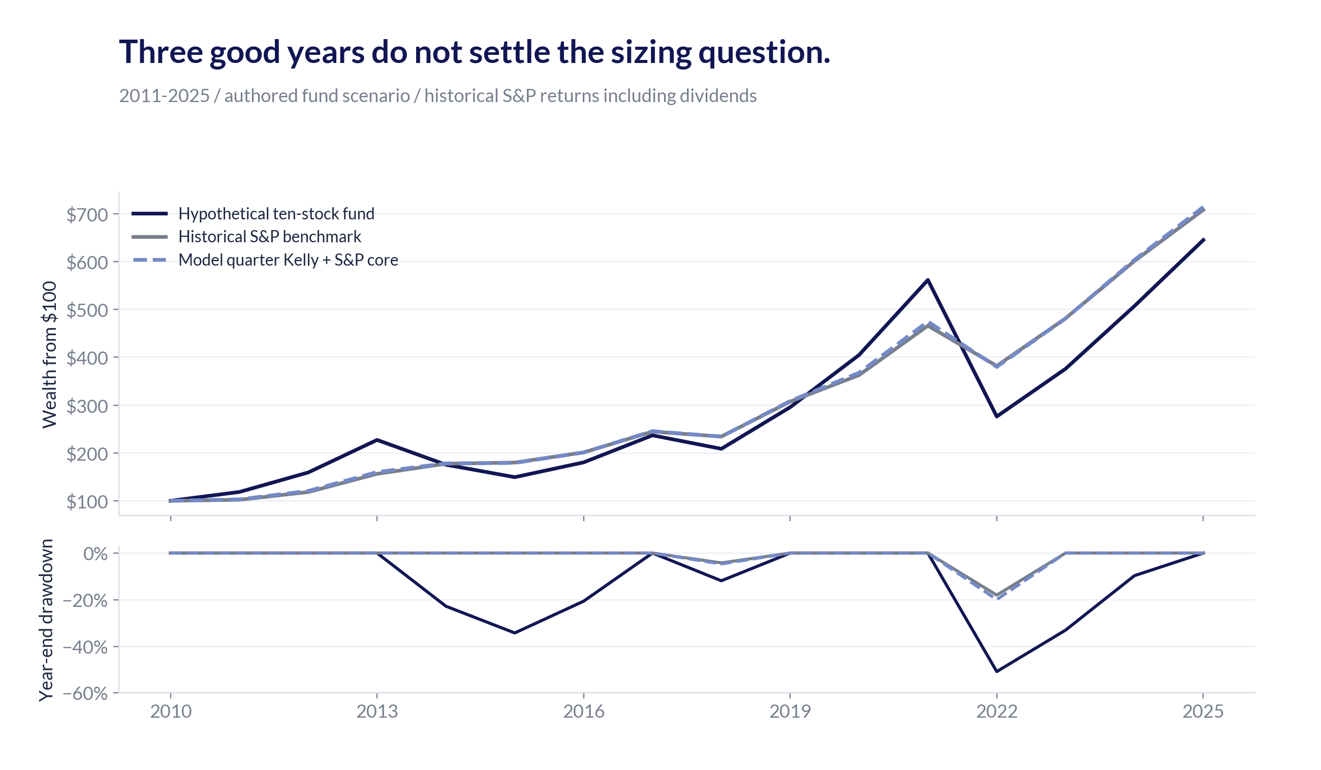
At first glance the final result looks like a modest shortfall. The risk tells a different story.
| 2011–2025 | S&P benchmark | Ten-stock fund | Model quarter Kelly + S&P core |
|---|---|---|---|
| Annualized compound return | 13.94% | 13.23% | 14.01% |
| Annual-return volatility | 14.26% | 28.64% | 14.90% |
| Sharpe ratio | 0.95 | 0.56 | 0.91 |
| Worst year-end drawdown | −18.04% | −50.82% | −19.95% |
| Calmar-style year-end proxy | 0.77 | 0.26 | 0.70 |
All measures use 15 annual observations. Sharpe compares return above a Treasury-bill proxy with the variability of that excess return. The Calmar-style proxy divides full-period compound return by the worst year-end drawdown; it is not a standard monthly or daily Calmar ratio.
The manager takes roughly twice the volatility, suffers a much deeper loss, and finishes behind. Recovering from the 50.8% drawdown requires a gain of about 103%. The benchmark needs about 22% after its worst year-end decline.
Think of edge as revenue, volatility's drag on compounding as the cost of goods sold, and the return left for the investor as profit. Finding an edge is only half the job. Taking too much risk can eat the margin. A manager who talks only about the edge is like a business owner who brags about sales and forgets to check whether the company makes any money.
The quarter-sized version keeps substantial market risk. Its better result here does not establish that quarter Kelly always beats the market. It shows the effect of asking a modest stock-picking edge to do a modest amount of work.
Real managers have taken this ride
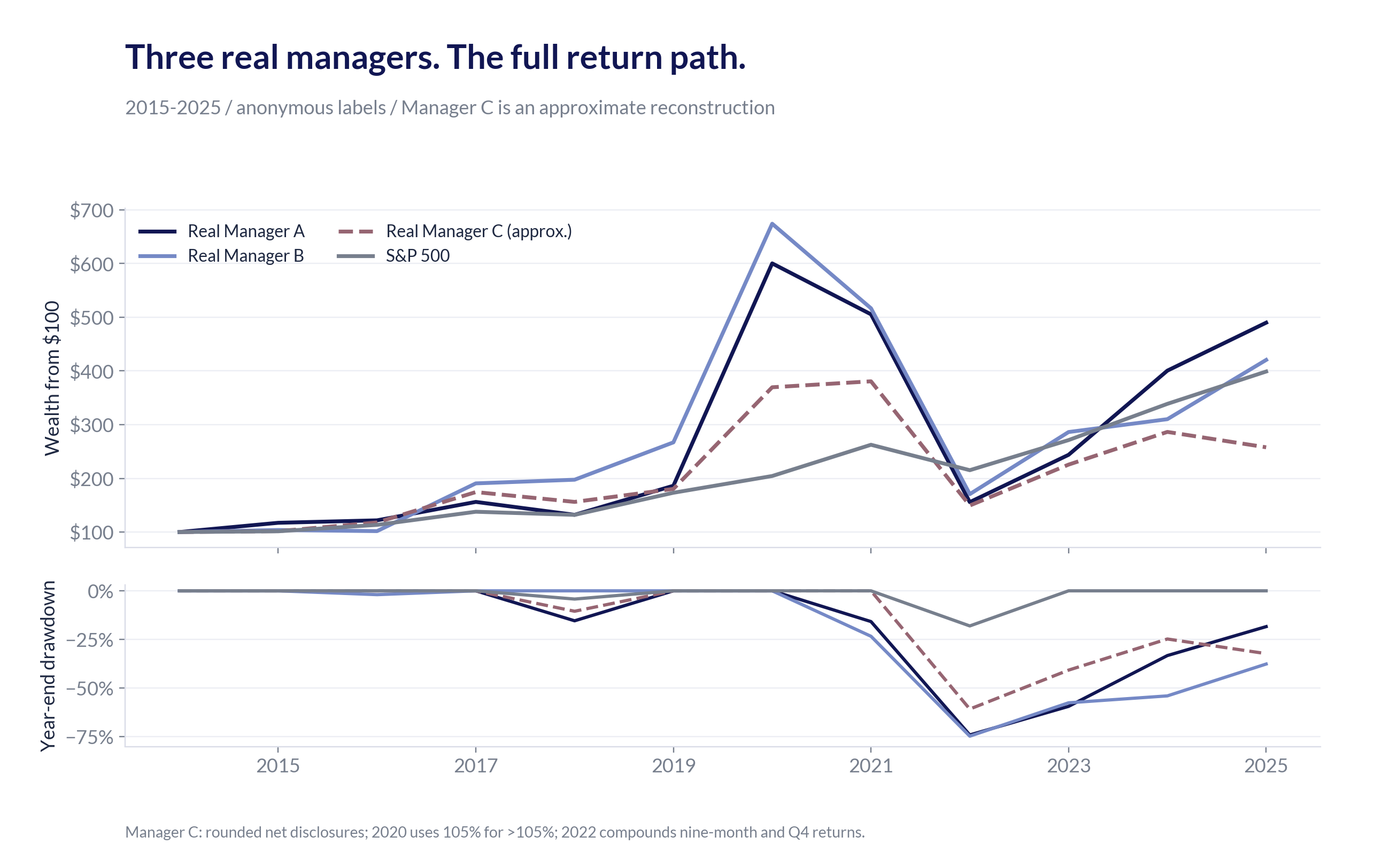
The following cases are real managers, kept anonymous because the argument concerns portfolio choices, not personalities. The complete return windows include their later recoveries.
Manager A gained 222.4% in 2020. Manager B gained 152.5%. In 2022 they lost 69.2% and 67.0%, respectively. Including losses in the prior year, each suffered a year-end peak-to-trough decline of roughly 74%–75%.
Both subsequently had large rebounds. Across the full 2015–2025 period, both finished ahead of the S&P benchmark in compound return. That makes the example more useful. A good ending does not erase the risk taken to reach it.
Manager C earned more than 105% in 2020. Its published, rounded figures imply a loss of about 61% in 2022, followed by gains of about 51% in 2023 and 27% in 2024, then a 10% loss in 2025. A large rebound and a full recovery are different things.
| 2015–2025 | S&P benchmark | Manager A | Manager B | Manager C (approx.) |
|---|---|---|---|---|
| Annualized compound return | 13.40% | 15.54% | 13.95% | ≈9.0% |
| Annual-return volatility | 15.42% | 73.40% | 59.04% | ≈42.3% |
| Sharpe ratio | 0.82 | 0.41 | 0.43 | ≈0.35 |
| Worst year-end drawdown | −18.04% | −74.07% | −74.70% | ≈−60.8% |
| Calmar-style year-end proxy | 0.74 | 0.21 | 0.19 | ≈0.15 |
These estimates use only 11 annual inputs and the same metric definitions as above. Manager C's figures describe the approximate reconstructed series, not an audited NAV history. Daily drawdowns can be worse. All three took much more risk than the market; the first two finished ahead, while the third reconstruction finished behind.
The two managers' annual returns had a correlation of about 0.88. Remove 2020 and 2022 and it falls to about 0.56. That small sample does not prove identical portfolios. It does challenge the idea that buying two different stories necessarily buys two independent sources of risk.
Manager C's own letters described concentration and shared exposure to growth and interest rates. Five holdings disclosed at the end of 2021 had an average daily return correlation of about 0.65 during 2022. Every pair exceeded 0.55.
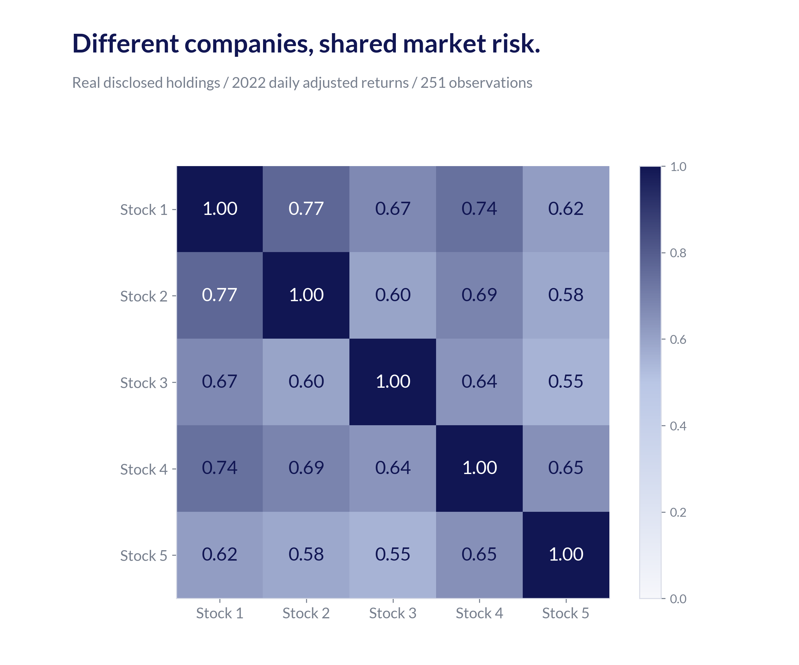
The precise ex-ante Kelly size of these real portfolios is unknown. Their true edge was never handed to us in a sealed envelope. What we can observe is concentration, shared risk, very large losses, and recoveries that required investors to stay invested.
The investor does not arrive at the start of the chart
When does a manager attract attention? Often after the spectacular run. When does an investor begin to doubt the strategy? Often after the spectacular loss.
The investor buys the impressive track record. Then he has to live through the next part.
Consider an illustrative investor who puts $100 with Manager A at the end of 2020, after that 222.4% year. The reported 2021 and 2022 returns turn it into about $26. If the investor redeems then, the later recovery belongs to somebody else. Even an investor who stays through the end of 2025 has about $82 from that entry point, despite the attractive full-window chart.
For Manager B, the same hypothetical entry and exit leave about $25 after 2022, or about $62 if held through 2025. These are calculations from the reported fund returns, not claims about what either manager's average client actually did.
For Manager C, the rounded return reconstruction puts the same hypothetical $100 entry at about $40 after 2022 and $70 after 2025. Again, these are illustrative entry dates, not records of actual client transactions.
Buy after the applause. Redeem after the explanation. The presentation keeps its long-term record; the investor keeps the loss.
There is broader evidence that cash-flow timing matters. Morningstar's 2026 study estimates that the average dollar in US mutual funds and ETFs earned about 1.2 percentage points less per year than their aggregate total returns over the decade ended 2025. More volatile funds tended to have wider gaps. That measures dollars and cash flows, not the behavior of a typical individual; it does not establish panic as the cause of every gap.
A deep drawdown is a financial problem and a test of whether the investor can keep holding. A fund manager cannot make that problem disappear by defining it as temporary. Redemptions can also create pressure to sell holdings at poor prices, especially when those holdings are illiquid.
The investor's staying power belongs in the sizing decision before the loss, not in a letter explaining it afterward.
The manager celebrated for holding CVNA
Consider another real manager: one who famously made a huge bet on CVNA and has been celebrated for the “conviction” to hold through the wild ride. A 2025 interview promoted the story as a lesson in conviction investing after the stock's collapse and extraordinary recovery.
The manager's April 2022 letter reported eight long positions. CVNA was 25% of capital at March-end; the second-largest holding was another 24%. By the letter's date, the portfolio was down about 43% for the year. This was a large commitment to a small group of businesses while losses were already severe.
The business survived and the shares staged a remarkable comeback. That recovery deserves to be included. It also creates a tempting shortcut: the manager held, the stock recovered, therefore the original size was wise.
The conclusion does not follow. A successful outcome alone cannot establish that the probability of success justified the amount at risk. We also need to ask what could have happened, how much permanent loss was possible, and how many investors could remain invested through the decline.
We do not have the client cash-flow records to say how many bought near the high or redeemed near the low. The question still matters. A recovery rewards the dollars that remain invested. It cannot repair a loss for an investor who has already left.
The survivor gets the interview. Investors who could not survive the ride are missing from the story.
Humility should change the portfolio
Kelly asks us to connect belief to money. Quarter Kelly adds an allowance for the fact that our beliefs can be wrong.
Before making a large position, write down the expected payoff, the plausible downside, and the evidence for the advantage. Check how often similar forecasts were right. Ask what would change the estimate. Then count the shared risks across the entire portfolio.
Stress the assumptions. Make the edge smaller. Make the loss larger. Let correlations rise when funding gets tight. Consider the investor who arrives after the best year and needs money after the worst one. If the portfolio only makes sense when every estimate is right, the position sizes are doing too much.
Company research and portfolio construction have different jobs. One looks for an advantage. The other decides how much damage a mistaken estimate is allowed to do.
Humility that leaves the weights unchanged is easy to market. The useful kind makes the bet smaller.
Calculation notes and data
Betting examples
For independent even-money bets with known win probability p, full Kelly is f = 2p − 1. With fractional scaling c, the stake is c(2p − 1). Expected log growth is p ln(1 + f) + (1 − p) ln(1 − f). At true p = 0.52, a 10% stake makes this negative. With exactly 520 wins and 480 losses, terminal wealth is 100(1 + f)^520(1 − f)^480. The plotted ordering is fixed; terminal values depend on the counts. These are pedagogical examples, not stock-weight recommendations.
For an isolated stock returning either +u or −d against zero-interest cash, full Kelly weight is [pu − (1 − p)d] / (ud). With u = d = 0.40, quarter weight 10% implies full weight 40% and p = 0.58. The 95% Wilson interval for 55 successes in 100 independent trials is approximately 45.25%–64.39%. Dependence or changing conditions make a literal repeated-trial interpretation harder.
Ten-stock model and correlation
Each pick's gross return is (1 + benchmark return)(1 ± 0.40), with a 53% marginal probability of the positive sign. With probability 60%, all picks share one sign; otherwise signs are independent. This makes pairwise residual-sign correlation exactly 0.60. It is not an estimate of actual managers' skill or their total stock-return correlation.
The equal-weight pick sleeve has weight x, with the remainder in the benchmark. Full sizing maximizes expected relative log growth E[ln(1 + x e)] over this sleeve and benchmark mix, where e is the sleeve's relative return. It yields x = 0.2334087; quarter sizing is 0.0583522. This is a constrained model solution, not an unrestricted optimum for all investments. Annual winner counts are authored as 7, 7, 6, 1, 3, 6, 6, 4, 6, 7, 6, 0, 6, 6, 6. The path was designed to show early success and later shared losses. Annual rebalancing is assumed. Hypothetical returns exclude fees, taxes, costs, leverage, and cash flows.
For equal weights, equal standalone risk, and common pairwise correlation r, the variance-equivalent independent-bet count is N / [1 + (N − 1)r]. It describes diversification under those assumptions, not the number of distinct businesses or a complete factor model.
Return and risk measures
The S&P benchmark is NYU's compiled annual S&P 500 series including dividends, not a daily official total-return index. Compound return uses the full window. Volatility is the sample standard deviation of annual returns. Sharpe is the mean annual excess return divided by its sample standard deviation, using the saved annual three-month Treasury-bill observations. Year-end drawdowns use the running wealth peak, including the initial $100. The Calmar-style proxy is full-window CAGR divided by the absolute worst year-end drawdown. Annual sampling misses losses between year-ends; these proxies must not be compared with differently sampled metrics as though their definitions matched.
Manager A's reported series changes to a representative-account convention in 2021; client fee choices and outcomes vary. Manager B uses published fund NAV returns after expenses. Neither series establishes actual client money-weighted returns. The illustrative late entries apply reported 2021–2025 annual returns to $100 invested at the end of 2020, with no further flows. Public cases remain unnamed; identifying primary-source records are retained in the working research. CVNA's ticker is included at the author's request. Its case does not receive invented full-period risk statistics.
Manager C uses an approximate reconstruction of its main fund, not its separate fund-of-funds strategy. The 2015–2016 inputs come from a published presentation; 2016 was an unaudited net estimate under an earlier fee convention. Later inputs come from rounded annual letters and may reflect different fee classes. The 2020 letter says more than 105%; the chart uses 105% as a conservative proxy, not an exact return. The 2022 input is reconstructed as (1 − 0.59)(1 − 0.043) − 1, approximately −60.8%, using disclosed nine-month and Q4 net results. All Manager C statistics inherit those limits. This reconstruction cannot replace a continuous audited NAV series. No missing returns are taken from 13F values or from another fund.
Data: Historical benchmark observations, hypothetical annual returns and wealth, hypothetical risk calculations, and anonymous manager return inputs, including Manager C's reconstruction.